
Several years ago I collaborated with my friend and colleague, JMU mathematician (and all around 3D printing empress extraordinaire) Laura Taalman (known to many as mathgrrl) on a set of circle packing ornaments for Christmas. Recently, I saw this great video of the production of a lovely tesselation and saw our circle packing ornaments in the background of the video. It seems as good a time as any to write a tutorial on how you can make these yourself. This three part post is written in collaboration with Laura.
To follow along at home you will need (more for parts II and III):
- Jupyter Notebooks for coding the circle packing generation script and visualizing results. (Warning: the visualizations only work in the standard notebook interface, not in the new JupyterLab interface.)
- OpenSCAD for generating the printable STL files.
- koebepy for geometry processing and circle packing generation. (Warning: I have produced exactly zero documentation for koebepy. So far the only users of it are me and my students and I mostly use it for research. There is some information on how to install it here.)
- A love of geometry.
To actually obtain physical prints of your models you will need a 3D printer and slicer or you can use Shapeways to get very high quality prints. These models tend to be a bit hard to print at home on an FDM printer unless you make the circles rather beefy. We are able to obtain a particularly delicate result from Shapeways.
After writing the background for this post, we decided it would be best to split it into three parts. They are:
- Part I: What is a circle packing? Here we describe a little bit of background on what a circle packing is.
- Part II: Generating a random circle packing in koebepy. (Coming soon.) Here we show how to use koebepy to generate your own random circle packings like those visualized here in Part I.
- Part III: Producing the printable packing. (Alliterative! Coming soon.) Here we show how to output your circle packing from koebepy to OpenSCAD and make nice circles that print well (at least at Shapeways).
The rest of this post will be the background reading you need to fully appreciate Parts II and III. We will link to them here once they are completed.
All images for this post were created using koebepy.
What is a circle packing?
Suppose you have a pattern of interior disjoint circles in the plane. If two circles touch at their boundary we say they are in contact. The contact graph of a pattern of circles is the graph obtained by associating every circle in the pattern with a vertex/node of our graph and connecting two vertices by an edge whenever their corresponding circles are tangent. Figure 1 shows an example of a packing and its contact graph.

Now here we have drawn the contact graph by placing each vertex at the center of its respective circle and connecting up neighboring vertices by a straight line segment (that consequently passes through the point of tangency between the neighbors). However, you should not think of the contact graph as having any geometry per se. Instead it is simply a record of the combinatorial information (circle 1 is tangent to circles 2, 5, and 6; circle 2 is tangent to circles 3 and 4, etc.).
The circle pattern and contact graph above has a few additional special properties. First, every circle on the outer boundary is tangent internally to the same unfilled outer circle (this is the unit circle). Second, the graph is a planar graph and each face of the graph (other than the outer face) is a triangle, meaning that each face is a triple of mutually tangent circles. A circle pattern with this property, that all interior faces of the contact graph are triangles, is called a circle packing. Play with a couple of pennies on the table and place them in different contact graph configurations. You’ll soon start to notice special properties of packings of the pennies when the contact graph is formed entirely by triangles. We call a planar graph such that all interior faces are triangles a triangulation of its outer boundary polygon.
But now consider that one unshaded circle in figure 1 that encloses all of the others. Notice that it too is tangent to mutually tangent consecutive pairs of disks along the boundary of the packing. In other words, it is forming its own triangular pattern of contacts as well–just another set of triangles. This may be a little hard to see, so let’s move everything to the sphere by a stereographic projection.
Notice that our outer circle from figure 1 has become the equator in figure 2. (3D printed pen holder potential is strong with this one.) It might be nice to shrink that equator circle down a bit in a way that maintains all of the contacts. Turns out we can do this by applying a special map of the sphere to itself called a Möbius transformation.
There are lots of ways to think of these Möbius transformation maps, one is by pairs of stereographic projections from a sphere to a plane to a different sphere. (This video gives a really nice visualization of this view of Möbius transformations.) Another is that a Möbius transformation is given by applying an even number of circle inversions (we will use this view in Part II, and is why this area is sometimes called inversive geometry). The bottom line is that Möbius transformations map circles to circles and maintain contact graphs so we can get different “views” of our circle pattern by applying a Möbius transformation, or equivalently, by applying an even number of circle inversions. (An odd number of inversions works too, but flips the orientation, so counterlcockwise turns become clockwise, and vice versa.)
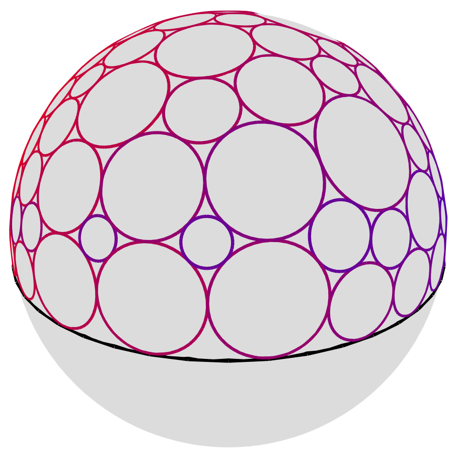
We’ll see how to do this in code later, but for now here’s the image of the circle packing from figure 2 after applying a Möbius transformation designed to shrink that equator down a bit.
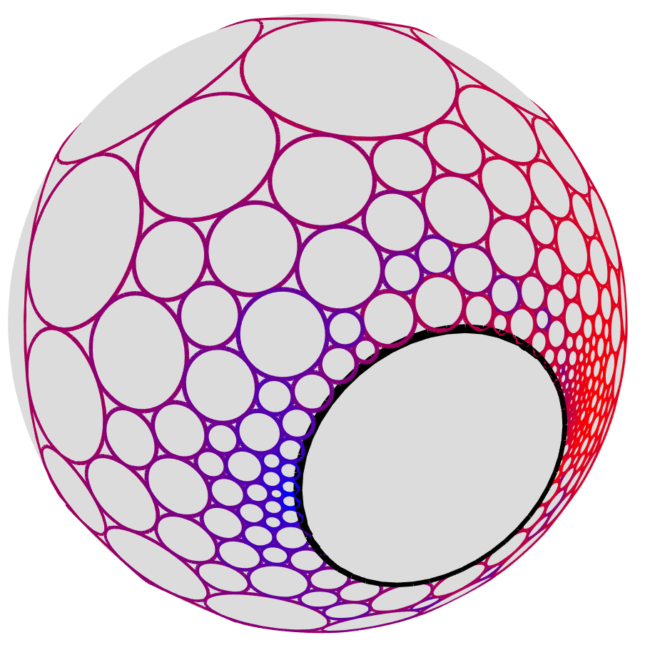
The sphere in figure 3 is rotated so that you can see where the entire lower hemisphere was mapped (the bigger circle with the black border–not close to an equator anymore). It got quite a bit smaller, and now the other circles are covering more of the sphere. Let’s visualize the contact graph:

Here we’ve added a visualization of the contact graph by placing the vertex corresponding to each circle outside the sphere at a special point called that circle’s conical cap. This point is the unique point in 3D euclidean space that is the apex of a cone tangent to the sphere exactly along the circle. We’ve then connected up conical caps of neighboring circles by 3D line segments connecting their conical caps. These segments have the special property that they are tangent to the sphere at precisely the point of tangency between the circles corresponding to their endpoints. The resulting triangulated polyhedron, which we call the Koebe polyhedron (named after the mathematician Paul Koebe who first worked with these objects) cages the sphere. Notice that here it is plain to see how the contacts between our original circle pattern (the shaded disks) and the outer unfilled circle (which became the equator and then shrunk down by a Möbius transformation) is actually a triangulation of the entire sphere.
So far we’ve started with a pattern of circles and from it derived its contact graph, which in our case was a triangulation, and looked at several different views of it, and noted that it forms a triangulation of a sphere. But what if we want to go in the reverse order. Suppose instead we know how many contacts we want and how we want them arranged into triangles so that the resulting triangulation is topologically equivalent to (i.e. homeomorphic to) a sphere? Can we get a pattern of circles that satisfy our contraints? It turns out that we always can. This was proven by Paul Koebe and later appeared in the work of E. M. Andre’ev and even later was used and popularized by Bill Thurston as a tool for studying hyperbolic 3-manifolds.
I’m going to state the important theorem a bit loosely, but the interested reader should check out [3] for a concise introduction, [4] for a book-length exploration of its properties and connections to harmonic analysis, and [2] for an overview of it, its generalizations, and lots of related results in the fascinating study of hyperbolic polyhedra. (Full disclosure: that last reference was written by John’s father and collaborator, Phil Bowers.) Anyway, here’s the relevant theorem, sometimes erroneously referred to as the Koebe-Andre’ev-Thurston theorem (which is a more general theorem that allows for overlapping circles of which this version is a special case–oh, and if you want to see some more about this theorem, check out John’s recent paper [1], ;-D). Anyways, here’s the relevant theorem:
Theorem 1. (The Circle Packing Theorem.) There exists a circle packing for any desired triangulated contact graph that is a sphere (is homeomorphic to a sphere). Furthermore, this circle packing is unique up to Möbius transformations.
This theorem says that we can choose any triangulation of a sphere we want and there exists a circle packing realizing it as its contact graph. Here’s an additional fun fact: by an appropriate Möbius transformation any of the circles in the pattern can be moved to the lower hemisphere and the stereographic projection of the resulting pattern will be like figure 1 with all of the other circles projecting to circles on the interior of a single outer circle. This is interesting because it means we can circle pack triangulations of disks as well.
Theorem 1, slightly revised. (The Circle Packing Theorem for Disks.) There exists a circle packing for any desired triangulated contact graph that is a disk (is homemorphic to a disk) with all of its outer circles internally tangent to the unit circle. Furthermore, this circle packing is unique up to Möbius transformations that map the interior of the unit disk to itself.
Finally, we note that if we think of the interior of the unit disk as the Poincaré disk model of the hyperbolic plane 
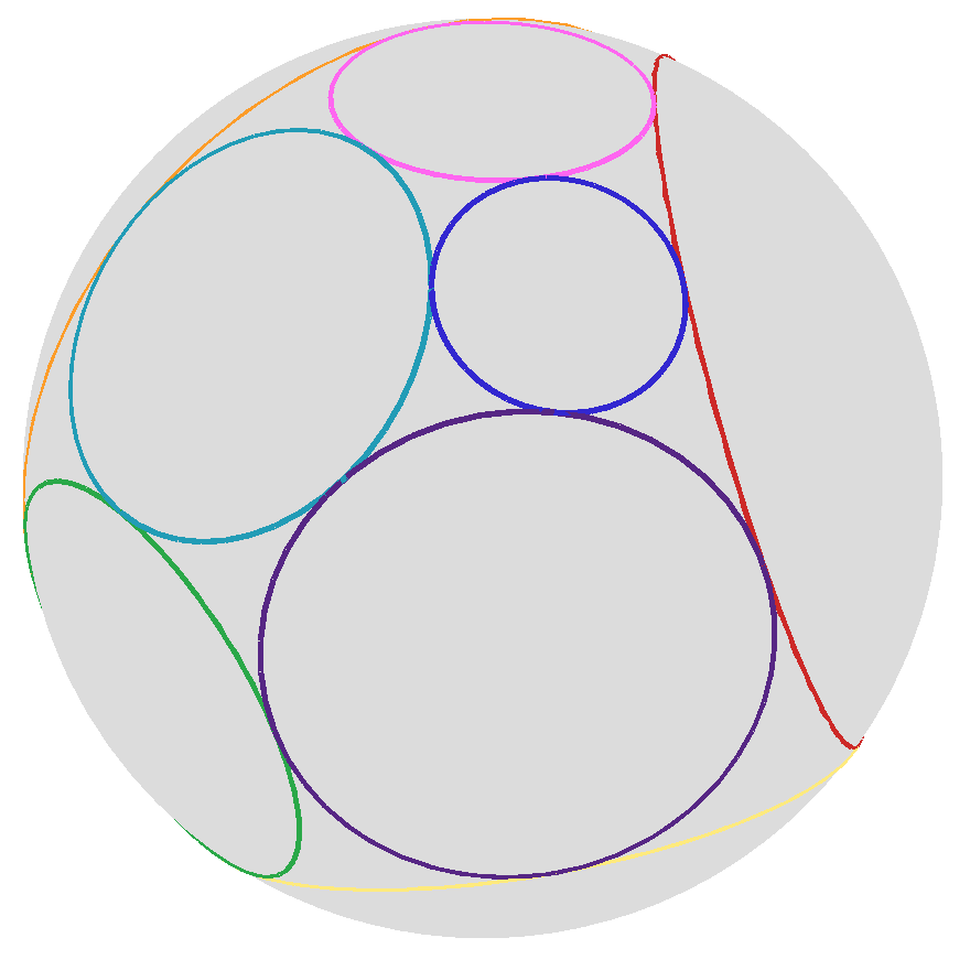
Furthermore, there exist algorithms that take as input a desired contact graph and produce as output a circle packing. In other words, given this:

A circle packing algorithm will produce this (or a Möbius transformation of it):
This is enough background. See references [2, 3, 4] for more information. We will now turn to using the koebepy library and OpenSCAD to create 3D printable circle packing ornaments.
That’s enough background for circle packing ornaments. In Part II we will use koebepy to generate random circle packings and in Parti III we’ll turn them into printable models. Stay tuned.
References
[1] John C. Bowers. A proof of the Koebe-Andre’ev-Thurston theorem via flow from tangency packings. Preprint. ArXiV 2007.02403
[2] Philip L. Bowers. Combinatorics encoding geometry: The legacy of Bill Thurston in the story of one theorem. In K. Ohshika and A. Papadopoulos, editors, In the tradition of Thurston: geometry and topology. Springer, 2020
[3] Kenneth Stephenson. Circle packing: A mathematical tale. Notices of the American Mathematical Society, 50(11), pp. 1376-1388, 2003. (pdf)
[4] Kenneth Stephenson. Introduction to Circle Packing: the Theory of Discrete Analytic Functions. Camb. Univ. Press, New York, 2005. (ISBN 0-521-82356-0, QA640.7.S74)
