Make Your Own Circle Packing Ornaments Part II: Generating a random circle packing in koebepy.

This post is part II of a three part series. Several years ago I collaborated with my friend and colleague, JMU mathematician (and all around 3D printing empress extraordinaire) Laura Taalman (known to many as mathgrrl) on a set of circle packing ornaments for Christmas. Recently, I saw this great video of the production of a lovely tesselation and saw our circle packing ornaments in the background of the video. It seems as good a time as any to write a tutorial on how you can make these yourself. This three part post is written in collaboration with Laura.

This is Part II of a three part series.

• Back to Part I: What is a circle packing?
• Onward to Part III: Producing the printable packing. (Coming soon.)

To follow along at home for this part you will need Jupyter notebooks and koebepy running.

All images and the video for this post were created using koebepy. A Jupyter notebook containing all the code for this post is available at the end under the “Files” heading.

Overview of the ornament generation algorithm

The circle packing theorem, as described in part I, guarantees that if we have a triangulation of a sphere there exists a circle packing whose tangency graph is our triangulation. Furthermore, there are known algorithms for computing circle packings from a given triangulation (maybe a future post could discuss some of these). As we saw in part I, an algorithm that can pack the interior of the unit disk, or equivalently produce a maximal packing of the hyperbolic plane in the Poincare disk model, can be used to produce circle packings for the sphere as well. We simply stereographically project the pattern back to the sphere. This is good, because there aren’t really any algorithms for computing circle packings on the sphere itself. All of them either pack in the Euclidean plane, or produce packings in the hyperbolic plane. Koebepy implements an algorithm for circle packing on the hyperbolic plane, which is simply a translation into Python of a Java version from Ken Stephenson’s fully featured, open source circle packing application CirclePack. The main steps of the algorithm are as follows.

1. Generate a random triangulation that is homeomorphic to a sphere (i.e. a polyhedron made up entirely of triangles).
2. Remove one face of the polyhedron (poke a hole in it, essentially) to make it a disk.
3. Use the hyperbolic circle packing algorithm to maximally pack the hyperbolic plane and realize it as a set of circles in the Poincaré disk model of the situated in the unit disk in the Euclidean plane .
4. Stereographically project this back to the sphere.
5. Find and apply a Möbius transformation that makes our circle packing look pleasing.

Along the way we will use a couple of tools from koebepy that make the code very easy. Koebepy already has routines for generating random triangulations, data structures for representing triangle meshes and modifying them via operations like removing a vertex, producing hyperbolic circle packings, etc. It also has a lot of geometric objects that allow us to do easy synthetic geometry in code. Currently, because it was developed by John to support his own idiosyncratic research, there is nearly no documentation anywhere available (this really needs to be fixed, and its on the todo list), but this post will expound on some of the design of koebepy as we go. Koebepy also has facilities for visualization within a Jupyter notebook and animations. These are built on top of the p5.js JavaScript Processing library, but you don’t have to know anything about Processing or JavaScript to use them. The goal of koebepy’s visualization interface is ease-of-use over power. It provides essentially none of the typical graphics tools. You just tell it what geometric objects you want drawn, and it draws them for you. Think of it more like a code version of Geogebra (although it doesn’t even implement an object dependency graph) than a full fledged graphics library.

Generating and viewing a random triangulation

Ok, so let’s get started. The first thing we need to do is generate a random triangulation. The algorithm that koebepy implements for this is really simple. Given a desired number of vertices , koebepy uniformly samples the unit sphere times to come up with a set of 3D points. It then computes the convex hull . The convex hull is the smallest convex polyhedron containing all the points and has the property that (generically) the vertices of the polyhedron are precisely the points in ., since all our points are on the sphere and the sphere is itself convex. The word “generically” here means that this property holds so long as no four of our points happen to lie on the same plane in . This occurs with probability zero (of course since we’re doing this on a computer and are thus using a pseudorandom number generator, the probability isn’t exactly zero, but it is very, very small). Also generically, the faces of the convex hull are all triangles, so this method (with high probability) produces a polyhedron with vertices comprised entirely of triangles. Exactly what we need!

Here’s the koebepy code to produce the random triangulation with some inline comments.

from koebe.algorithms.incrementalConvexHull import randomConvexHullE3

N = 100 # The number of vertices we want

# Get a random convex polyhedron with N vertices:
rando = randomConvexHullE3(N) 

That’s it!

A couple of side notes. First, koebe.algorithms is where koebepy stores algorithms for computing geometric things and koebe.algorithms.incrementalConvexHull is where the convex hull algorithm is implemented along with some related algorithms like the random generation of convex polyhedra we are using here, randomConvexHullE3. Also, note the “E3” at the end of that name. That stands for , the Euclidean 3-space. Koebepy stores geometric objects in seven different geometries, the standard Euclidean 2D and 3D geometries and , as well as the hyperbolic plane , the extended complex plane (also known as the Riemann sphere), oriented projective 2 and 3-space, and the unit sphere . Except in the case of the extended complex numbers, objects are coded with a suffix for whatever geometry they live in. For example, PointE2, PointE3, and PointS2 represent points in the Euclidean plane, Euclidean space, and on the unit sphere (respectively). There are also lots of conversions implemented between them. For instance, if you have a PointE2 in the Euclidean plane you can convert it to a PointOP2 in the oriented projective plane (don’t worry if you don’t know what that is) by calling the toPointOP2() method. These conversion methods have been added as they’ve been needed, so there isn’t always a direct conversion. Sometimes you use an intermediate geometry to tie these together. This is a little annoying, so feel free to add ones you need and send a pull request on the koebepy GitHub. The geometry objects are all stored in the koebe.geometries package if you want to look around.

So now, how can we visualize it? Koebe’s visualization is built around the notion of a sketch viewer, which is a window into a particular geometry. The basic idea is that you construct a viewer object, you tell it what geometric objects you want to draw, and then you ask it to show itself. You can optionally add style information, which we’ll discuss later. For now, here’s how to sketch our random polyhedron.

from koebe.graphics.euclidean3viewer import E3Viewer

# Create a 600x600 pixel viewer
viewer = E3Viewer(600, 600)

# Add the rando polyhedron to the viewer
viewer.add(rando)

# Show the viewer
viewer.show()

Easy again! Here’s what ours looks like:

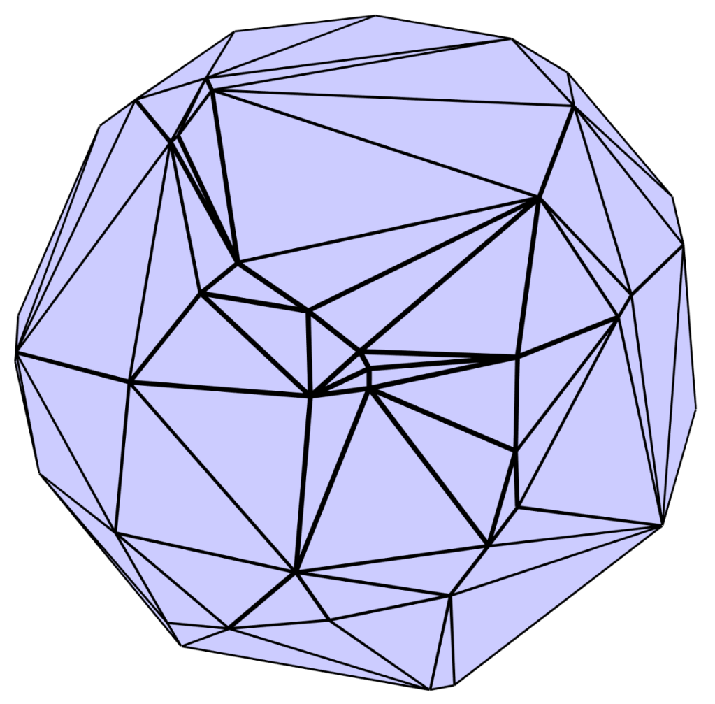
The Jupyter notebook version of this is completely interactive–you can click and drag to rotate the view and use the mousewheel to zoom in/out. Once you are done viewing it, it is a good idea to comment out the viewer.show() line and rerun the code block to hide the visualization. I find that if I have too many simultaneous 3D visualizations running it can slow the Jupyter notebook down a little and its best to only have one running at a time. The 2D visualizations are not animating by default (the 3D are even if nothing is moving to allow for the mouse rotations) so this isn’t necessary for 2D views.

Circle packing our triangulation

The data structure that stores our polyhedron is called a doubly-connected edge list (DCEL) data structure. It is a standard data structure in computational geometry and stores a lot of topological information about a polyhedron and supports many queries efficiently. For example, we can easily start at a vertex and collect all of the edges incident to it, or all of the faces (triangles) incident to it. Or we can start in a face, and ask for all neighboring faces. Etc. They are a little complicated the first time you see them, but we won’t really need to get into their details here. The main property we need right now is how to convert our polyhedron into a disk. We could remove a vertex and add it back later, but an easier trick is to just turn one of the faces into a hole in the mesh. The DCEL represents a disk by specifying one special face as an “outer face”, which sort of means non-existent face. This is used to track the boundary of the disk. For our purposes however, it makes it really easy to convert our disk from something that is topologically a sphere and closed, to a disk. Just select any face as the outer face (in our case we’ll just use the face at index 0). To do this we add the following code.

# Make the 0 index face the outer face
rando.outerFace = rando.faces[0]

Now let’s circle pack it. We use the hyperbolic packing algorithm.

from koebe.algorithms.hypPacker import maximalPacking

packing, _ = maximalPacking(rando)

The maximalPacking function returns two things: the packing data (as another DCEL) and the number of iterations it performed before numerical convergence. Since we only need the packing information, we use _ to ignore the other return value.

Let’s view the packing. Since this is a packing of hyperbolic space, viewing the packing in the Poincaré disk model is appropriate. To do this we create a PoincareDiskViewer viewer, add the circles from the packing to it, and then show the viewer. Because the Poincaré disk model is really sitting inside , this viewer is housed in the koebe.graphics.euclidean2viewer package.

There’s one catch here. The PoincareDiskViewer doesn’t know how to show a circle packing (we’ll get to it eventually), but it does know how to show circles. So we need to collect the list of circles from the packing object to send to the viewer. Each circle is associated with one vertex of the packing and this is stored in the .data attribute of the vertex. All the vertices are stored in a list as the .verts attribute of packing. For example, we can print out the first vertex’s data using:

print(packing.verts[0].data)

which prints something like:

CircleH2(center=PointH2(coord=ExtendedComplex(z=0j, w=(1+0j), _complex=None)), xRadius=0.007431371566812585)

In other words, we have a hyperbolic circle with a center and radius (xRadius comes from the way CirclePack implements circle packing; it is the Euclidean radius of the circle when drawn in the Poincaré disk model or its negative in the case of a horocycle). The center is given by a PointH2 object, which is a hyperbolic point. It’s coordinate is given by an extended complex number. An explanation of extended complex numbers is way beyond the scope of this writeup.

To collect all of the vertex data circles into one list we use a list comprehension, which is a programming feature in some languages (like Python) that mimics set builder notation from mathematics:

# Extract the .data attribute from each vertex in the packing:
circlesH2 = [v.data for v in packing.verts]

This time we have a list of geometric objects instead of just a single object we want to add to the viewer, so instead of using .add(obj) we need to use .addAll(objs) to add all of the objects in the circlesH2 list to the viewer. Here’s the code:

# Create a Poincare Disk Viewer
disk_viewer = PoincareDiskViewer(600, 600)

# Add all of our circles to it
disk_viewer.addAll(circlesH2)

# Show the viewer
disk_viewer.show()

And here is the resulting packing:

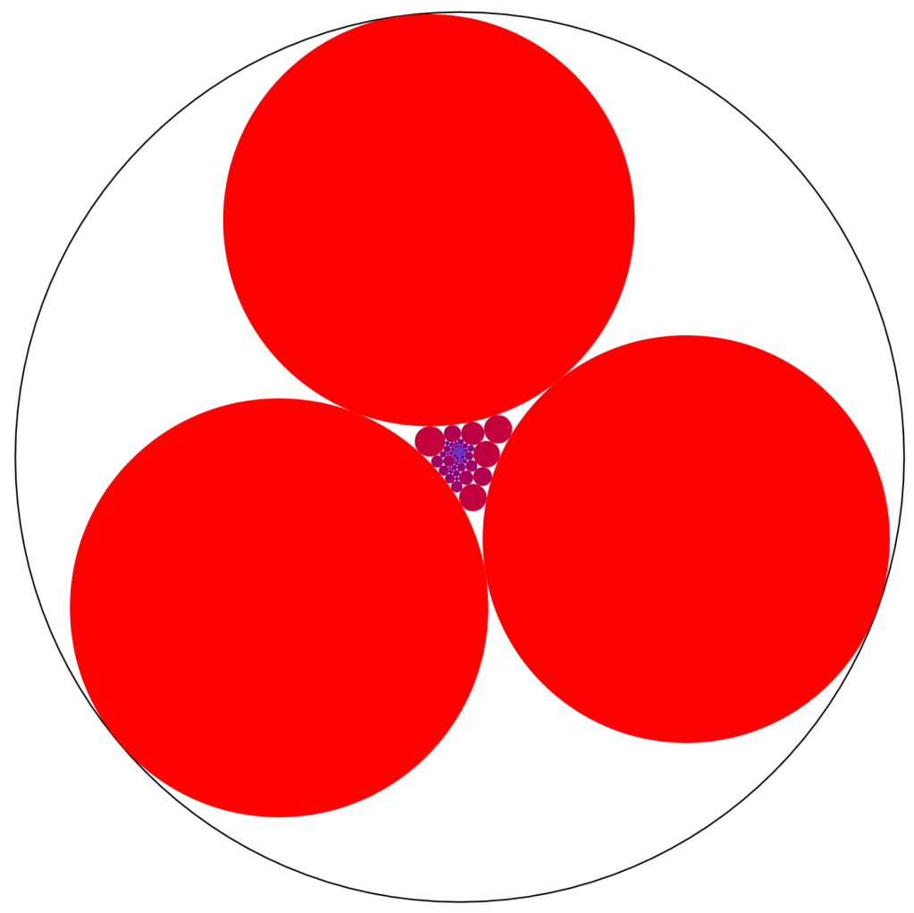
Pretty cool but a bit boring in black and white. Now seems as good a time as any show how to style/color it. There are several ways to style objects added to the viewer. When using .add we can optionally pass the style we want, as in viewer.add(object, style). When using .addAll we can style objects by sending a list of tuples where the first entry in each tuple is the object and the second entry is the style. Calling this version looks something like viewer.addAll([(obj1, style1), (obj2, style2), ...]) We could modify our generation of the circlesH2 list to do this. Finally, we can, after already adding an object to the viewer use the .setStyle(obj, style) to change its style. This is what we’ll do here. But how do we specify a style? This is done using the makeStyle function that can be imported from any of the viewers. We’ll have to modify the import statement that imports the PoincareDiskViewer slightly to accomplish this, so pay attention to that detail. The makeStyle function has three parameters, each of which are optional: stroke, the color specification for the pen stroke that draws the outline of the geometric object, strokeWeight, the thickness of the pen stroke (1.0 is equivalent to one pixel), and fill the fill color of an object. If either the stroke or fill colors are unspecified then they are ignored. The colors must be specified using standard CSS3 color specifications, which can be hex, like “#3300a0”, or color names, like “red”, or RGB values like “rgb(255, 12, 200)”, or RGBA values like “rgba(255, 12, 200, 0.5)”. To show off this feature a bit, I’m going to color each circle by its area. Here it is:

import math

# Extract the .data attribute from each vertex in the packing:
circlesH2 = [v.data for v in packing.verts]

# Note the additional import of makeStyle:
from koebe.graphics.euclidean2viewer import PoincareDiskViewer, makeStyle

# Create a Poincare Disk Viewer
disk_viewer = PoincareDiskViewer(600, 600)

# Add all of our circles to it
disk_viewer.addAll(circlesH2)

# Compute the absolute value of the natural log of 
# each radius (the circles look like they shrink 
# exponentially fast, so I wanted to linearlize
# this a bit)
logRadii = [abs(math.log(abs(c.xRadius))) for c in circlesH2]

# Set the style of each circle
# We will color the largest circles red, 
# the smallest blue, and then interpolate 
# exponentially between them.
for i in range(len(logRadii)):
    c = circlesH2[i]
    t = (logRadii[i] - min(logRadii)) / (max(logRadii) - min(logRadii))
    red = int(255 * (1 - t))
    blue = int(255 * t)
    disk_viewer.setStyle(c, makeStyle(fill=f"rgb({red}, 0, {blue})"))

# Show the viewer
disk_viewer.show()

And here’s the result:

Circle Representations

Let’s talk for a bit about circle representations. The CircleH2 object we’ve seen stores a circle as a center PointH2 object and a radius. Similarly, CircleE2 objects are stored this way with a center PointE2 object and a radius. This is not the only way to represent a circle. Another way is to use the homogeneous equation of a circle, which is

Here we represent a circle as the four coordinates . The equation is homogeneous, which means that scaling all the coefficients by a non-zero results in the same circle, so and represent exactly the same circle. Furthermore, we can use the sign of to determine a particular side of the circle. If we consider the circle to bound the disk on its interior. When , we consider the outside to be a disk (which happens to include the point . This may not make much sense here on the plane, but makes a lot of sense when we stereographically project to the sphere (because every circle has two “insides”–two disks that it bounds). This is the representation we use for the DiskOP2 class.

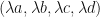
Finally, a circle on the sphere could be given by center and radius in spherical coordinates and lengths. Koebepy uses a different parameterization. Each circle on lies in a plane in that intersects at that circle. That plane is given by the homogeneous equation

.

So, as before, we can represent a circle on the sphere by a 4-tuple of coordinates and as before this circle is invariant under scaling; and are equivalent for . We’ll say the inside of the circle is the disk that the normal points towards. Thus multiplying by a negative lambda results in flipping which disk we are referring to.

The nice thing about this last view is that it becomes very easy to figure out the coordinates for certain disks. For example, a plane through the origin in always has . So the equator of the sphere is given by coordinates , which also denotes the upper hemisphere. The lower hemisphere is given by . The great circle contained in the -plane is . Furthermore, we can obtain less than great circles by varying the parameter on each of those equations. Here’s a quick sketch to show this.

from koebe.geometries.spherical2 import DiskS2
from koebe.graphics.spherical2viewer import S2Viewer, makeStyle

# Create two sets of disks, the a's and the b's
a1, a2, a3 = DiskS2(1, 0, 0, 0), DiskS2(1, 0, 0, 0.75), DiskS2(1, 0, 0, 0.25)
b1, b2, b3 = DiskS2(0, 1, 0, -0.25), DiskS2(0, 1, 0, 0), DiskS2(0, 1, 0, 0.25)

# Create a red and a blue style
redStyle = makeStyle(stroke="red", strokeWeight=2.0)
blueStyle = makeStyle(stroke="blue", strokeWeight = 4.0)

# Create a viewer for the sphere S2:
s2viewer = S2Viewer(600, 600)

# Add the a disks and style them red
s2viewer.addAll([(a1, redStyle), (a2, redStyle), (a3, redStyle)])

# Add the b disks and style them blue
s2viewer.addAll([(b1, blueStyle), (b2, blueStyle), (b3, blueStyle)])

s2viewer.show()

Which results in:

Projecting to the sphere and changing the view (via circle inversions)

Now let’s project our circles to the sphere and visualize them. The stereographic projection that is implemented in koebepy is a bit weird because instead of placing circles in the -plane for projection, it puts them into the -plane and projects to the lower hemisphere (let’s be clear, this is a bug not a feature). All we need to do is take each circle in and provide the necessary koebepy incancation to stereographically project them and finally add them to an S2Viewer. The problem is that there’s no direct conversion from a CircleH2 to a DiskS2. We have to use DiskOP2 as an intermediary. And there’s no direct conversion from CircleH2 to DiskOP2. We have to use CircleE2 as an intermediary. The idea is that we use the CircleH2::toPoincareCircleH2() to do the first conversion, which simply replaces the CircleH2 object with its Euclidean circle in the Poincaré disk representation. We then use the DiskOP2.fromCircleE2(circle) class method to convert the center/radius representation of the CircleE2 class into the homogeneous coordinates of the DiskOP2 class. We then use the toDiskS2()method of DiskOP2 to stereographically project this onto the sphere.

Here’s the code:

from koebe.geometries.orientedProjective2 import DiskOP2

disksS2 = [DiskOP2.fromCircleE2(c.toPoincareCircleE2()).toDiskS2()
           for c in circlesH2]

# Create a viewer for the sphere S2:
s2viewer2 = S2Viewer(600, 600)

# Add the a disks and style them red
s2viewer2.addAll(disksS2)

s2viewer2.show()

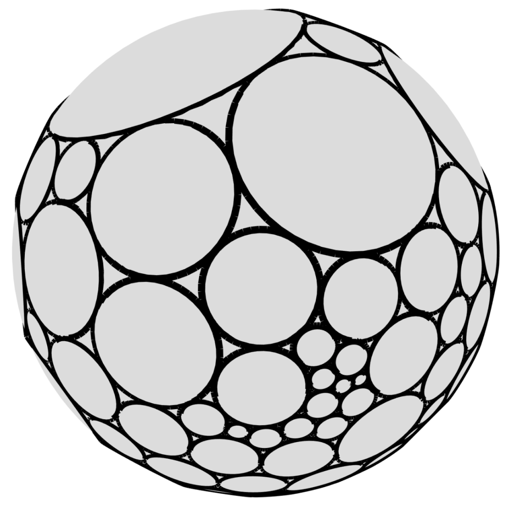
and here is the result:

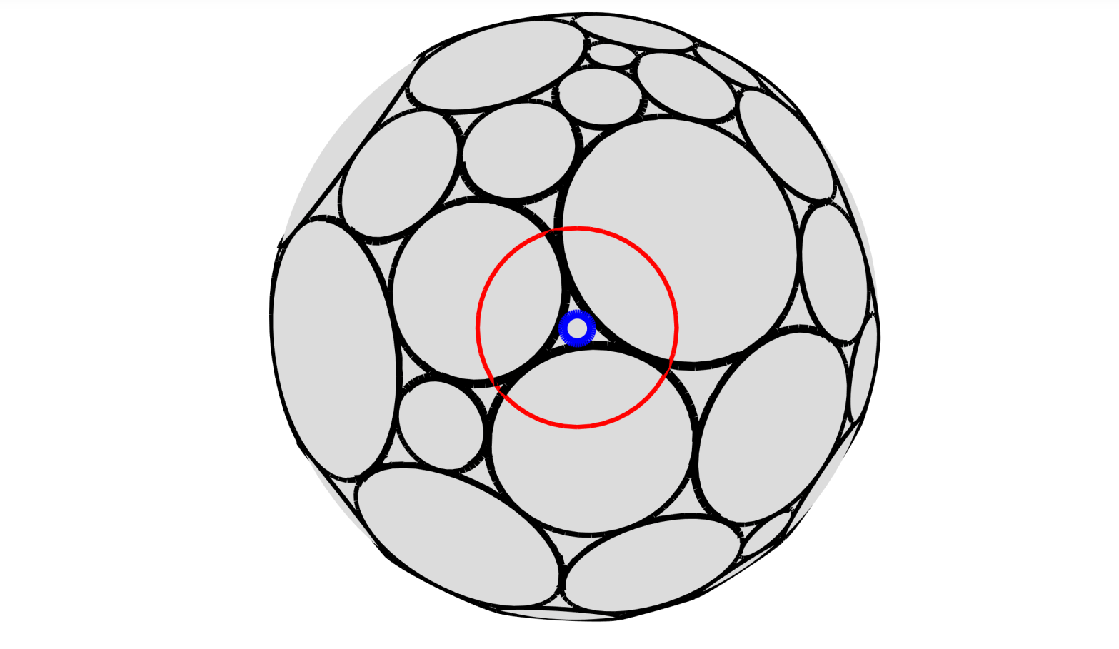
Ok, so we’ve now got it all on the sphere, but those three outer circles are huge and everything else is tiny. Not so ornamental. Fortunately, we can easily move these circles around using circle inversions, which are sort of like reflections through a plane in circle land. Since our circles were all projected into the positive -hemisphere of the sphere, we’ll select a circle parallel to the -plane in the lower hemisphere, invert through it, then select another similar circle and invert back.

Here are the two inversion disks:

I1 = DiskS2(1, 0, 0, 0.975)
I2 = DiskS2(1, 0, 0, 0.9995)

And here is adding them to the viewer and styling them:

s2viewer2.add(I1, redStyle)
s2viewer2.add(I2, blueStyle)

Here’s the result:

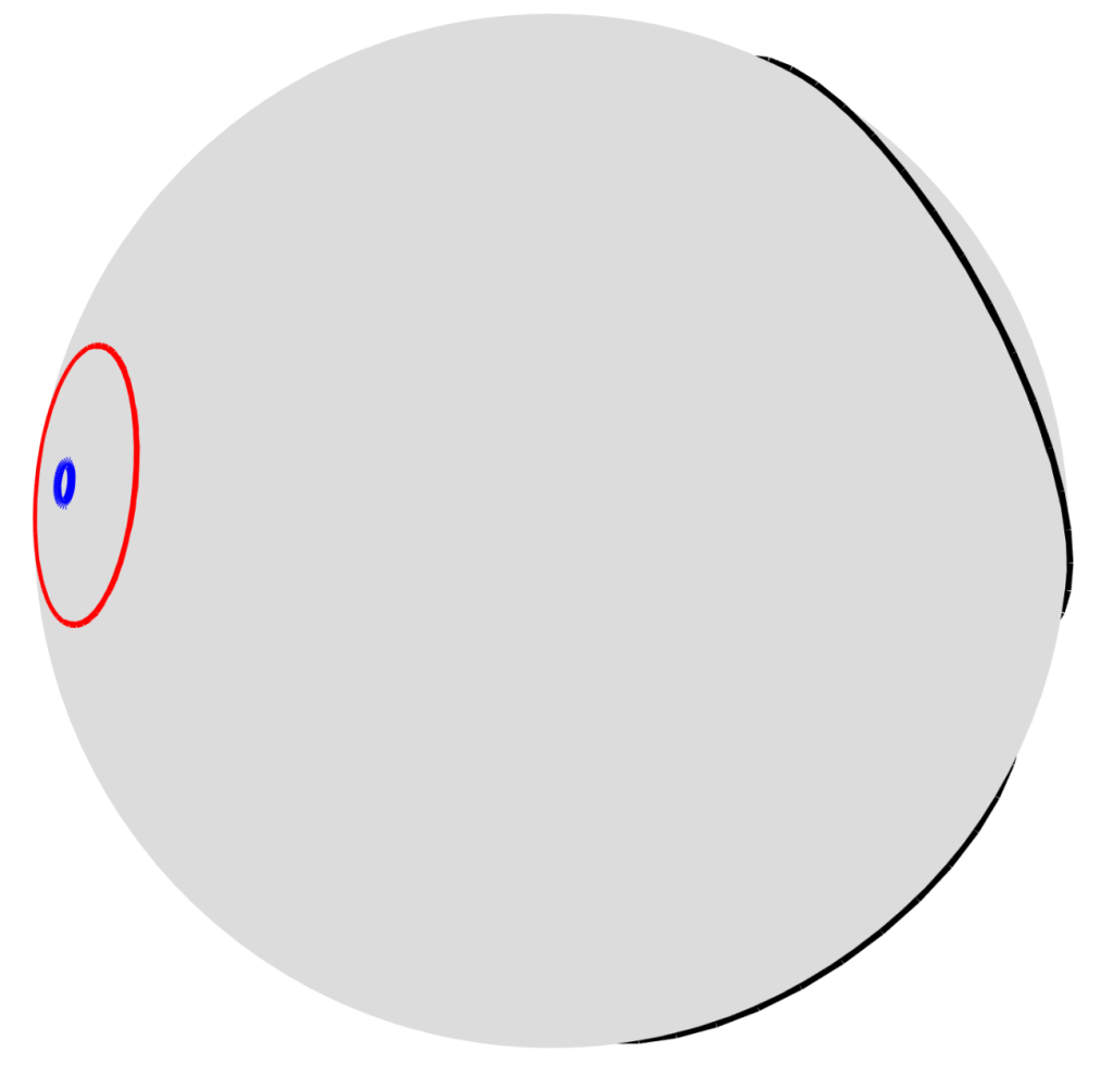
Now, we just need to perform the inversion. We’ll first invert through I1, then invert through I2. We’ll show the result of doing each of these separately. To invert through just I1 we cange the line of code that creates the disksS2 list to:

disksS2 = [DiskOP2.fromCircleE2(c.toPoincareCircleE2())
                  .toDiskS2().invertThrough(I1)
          for c in circlesH2]

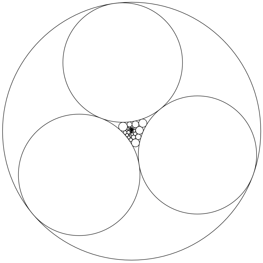
And now our circle packing is tiny and inside the blue circle:

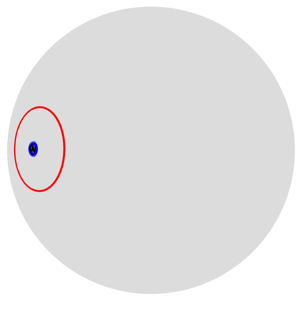
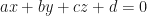
Finally, add the second inversion:

disksS2 = [DiskOP2.fromCircleE2(c.toPoincareCircleE2())
                  .toDiskS2().invertThrough(I1).invertThrough(I2)
          for c in circlesH2]

Now that is a pretty good looking circle packing, time to make some ornaments! The pair of circle inversions together gives us a Möbius transformation of the sphere. Any two circles can be chosen and will yield different results. We’re ready now for part III.

Bonus: Animation

As a quick bonus, it is really easy to produce animations in koebepy. Animations are done by providing the viewer with each frame of the animation and the viewer will automatically play them back in a loop. You set up each frame as if you are setting up the viewer as we have been doing above, except when you are done with a frame you call .pushAnimFrame() on the viewer to add a new blank frame after the current one. You can call this as many times as you want. The code below is a quick and dirty animation that interpolates the I1 disk from a great disk to the same as we chose above. Here’s the code:

from koebe.geometries.orientedProjective2 import DiskOP2

total_frames = 100

# We're doing an animation so we
# need to create the viewer before
# creating the geometry
s2viewer2 = S2Viewer(600, 600)

# loop over to generate each frame
for frame in range(total_frames):
    # if this isn't the first frame, 
    # push the last frame onto the frame
    # stack to get a fresh new frame to draw to
    if frame != 0:
        s2viewer2.pushAnimFrame()
    
    # I1's d coordinate is now based on what
    # frame we are on:
    I1 = DiskS2(1, 0, 0, 0.975 * frame / total_frames)
    I2 = DiskS2(1, 0, 0, 0.9995)

    disksS2 = [DiskOP2.fromCircleE2(c.toPoincareCircleE2())
                      .toDiskS2().invertThrough(I1).invertThrough(I2)
              for c in circlesH2]

    # Add the a disks and style them red
    s2viewer2.addAll(disksS2)
    s2viewer2.add(I1, redStyle)
    s2viewer2.add(I2, blueStyle)

s2viewer2.show()

Here’s the animation:

Files