Combinatorial tilings from finite subdivision rules

In this blog post I give an overview of infinite tilings generated using finite subdivision rules and show some koebepy that creates them. If you haven’t already, you may want to install koebepy. In a future post I plan to give a more in-depth tutorial on how to compute tilings using koebepy with this post serving as the necessary background.

This post gives a broad-strokes overview of combinatorial substitution tilings. The payoff at the end is a surprising theorem of R. Kenyon and K. Stephenson that shows the combinatorics of certain types of infinite tilings of the plain encode everything necessary to reconstruct their geometry. In other words, you can forget the geometry completely and play just a combinatorial game. Then compute a little conformal structure et voilá the geometry comes right back!

Nota Bene: The code used to produce the images in this blog post is built on the work of three of my fantastic former undergraduate students, Angelo Luna, Nicole Maguire, and Christian Fuller.

Introduction

A substitution tiling is a recursively defined structure in which we start with a set of one or more prototiles along with a finite subdivision rule for each prototile that defines how to cut each prototile up into a finite number of subtiles each of which is a (sort of) copy of one of the starter prototiles. I’m being informal here on purpose because we are going to look at two types of substitution tilings, geometric substitution tilings and combinatorial substitution tilings, and the precise meaning of subtile is a little different in each.

Geometric substitution tilings

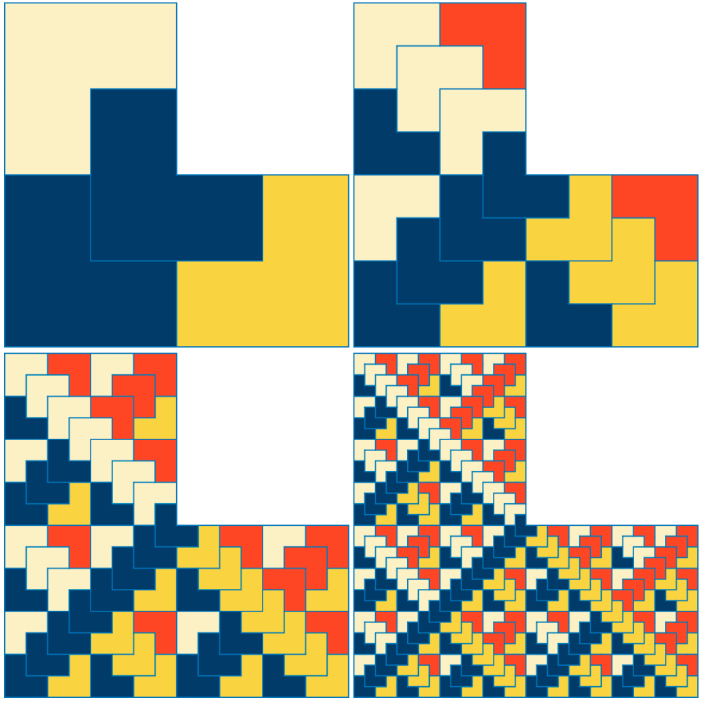
In a geometric substitution tiling each prototile has a specified geometric shape and the subdivision rule cuts the shape up into scaled and translated copies of the prototiles. Importantly, each subtile is scaled by the same constant factor. A nice example is the chair tiling. On the left of the figure below you can see a “chair” prototile and on the right you can see the chair’s subdivision into four smaller chairs, each exactly 1/2 the scale (and thus 1/4 the area) of the original. Technically, the chair tiling contains four prototiles and subdivision rules–the one shown below as well as its 90°, 180°, and 270° rotations. Below you see on the left the dark blue prototile, and on the right its subdivision into two 1/4 scale copies of itself (also in dark blue) as well as a 1/2 scale of its 90°-rotated (yellow) and 270°-rotated prototiles.

Once we have defined our prototiles and finite subdivision rules, we can produce subdivisions by starting with one of our prototiles as an initial tile and recursively applying the subdivision rules to all of the current tiles in the tiling. We say that the initial prototile is the level 0 tiling. Each time we recursively apply the subdivision rules we increase our level by +1. Here are several levels of the chair tiling.

Covering the plane via direct limits

Let us reproduce the same figure as above, except each time scaling the figure up by a factor of 2 so that the subtiles have the same size after subdivision as their parent supertiles did before subdivision.

In this case the tiling expands outwards from some scaling point. We continue this procedure each time selecting a scaling point on the interior of one of our tiles, subdividing all tiles by applying the appropriate subdivision rules, and then scaling everything out from our chosen scaling point. The limit of this procedure, which is called the direct limit, produces a geometric tiling of the entire plane into chairs in our case (or whatever tiles our tiling produces). The expansion of the chair tiling produces a special type of infinite tiling called an aperiodic tiling which lacks periodicity at any scale (a topic beyond our scope here). In fact, different choices of scaling point lead to different infinite aperiodic tilings of the plane giving us uncountably many ways to tile the plane aperiodically with chairs.

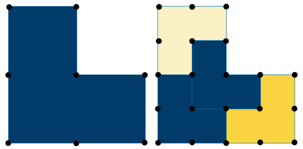
Now, it may seem like chairs have 6 sides and 6 corners; however, we have to be a bit careful here. Let’s look at the combinatorics of the tiling. Specifically, we’d like to think about the line segments that make up the tiling as edges in a planar graph. Vertices will be placed at the junction of multiple line segments in the subdivision. In the figure below I’ve placed large black circles representing the vertex at each junction. Can you spot the problem?

The problem is that though our dark blue tiles are geometrically similar they are not combinatorially similar. In fact, one is incident to 6 vertices (black circles) as we expected, but the other is incident to 8. This occurs because our subdivision rule matches one whole edge of the upper dark blue subtile with two other edges–one from the other dark blue subtile and one from the yellow subtile. One edge glued to two edges is throwing our combinatorics out of whack! From the point of view of our upper dark blue tile it sees one edge, but from the point of the view of the other blue and the yellow tile there are two edges. This simply cannot stand.

To fix this combinatorics-construction problem we will have to insist that combinatorially one edge is always just one edge, no matter which subtile’s point of view you are using to look at it. To fix the chair tiling’s combinatorics, because the subdivision rule seems to sometimes give rise to an octagonal chair, all chairs must be octagonal! Here’s the subdivision rule again annotated so that it shows the combinatorics:

Notice that now the prototile has been given 8 sides instead of 6. It just happens that two pairs of consecutive edges (namely along the left-hand side and bottom) are straight. Combinatorially, though, we don’t care about the geometry–we only care that we have an 8 sided shape. The subdivision rule now correctly divides the 8-sided chair up into four smaller 8-sided chairs. Importantly, in this version of the subdivision rule one edge is one edge–each edge is a full edge for both of the tiles incident to it. Everything is now consistent!

From geometric to combinatorial…

What if we forgot the geometry for the moment and focused on just the combinatorics? Technically we will think of a combinatorial tiling as a CW-complex homeomorphic to a disk. Essentially we want to forget the geometry and just focus on what discrete pieces make up the tiling. Consider our subdivision rule for the chair again, this time with the vertices labeled:

Let’s now describe this subdivision rule combinatorially. We begin with an 8-sided prototile ABCDEFGH. The subdivision rule requires 13 additional vertices a, b, c, d, e, f, g, h, i, j, k, l, and m. The first 8 additional vertices are obtained by splitting edges of the prototile. AB splits to obtain a, BC splits to obtain b, CD splits to obtain c, and so on. The final 5 vertices i through m are new vertices on the interior of ABCDEFGH. The tile is subdivided into four prototiles AaBjklHh, CcDdijBb, kjidEemlk, and GgHlmeFf. Is this all the information we need? Not quite. We need to know how the vertices of the prototile map to the vertices of a subtile. For example, in subtile kjidEemlk, which vertex is analogous to the the C vertex in the prototile? Look back at the previous figure. Clearly the i corner of the subtile matches up with the C vertex of the prototile. Let’s do another. Which prototile vertex corresponds to the m vertex of subtile GgHlmeFf? Well, the m is the the seat of the chair, so it corresponds to the E vertex of the prototile.

For each vertex in each subtile, we need to know which vertex it corresponds to in the prototile. To simplify the description we are going to require that each subtile be given in a consistent orientation. Notice that the order in which we specified each subtile above corresponded to a counter-clockwise walk around its boundary. Furthermore, we listed the vertices of each subtile in the same orientation and beginning with the same vertex as the corresponding orientation and vertices of its prototile. Thus, when we define CcDdijBb as a subtile whose prototile is ABCDEFGH we are implicitly defining the mapping from subtile to prototile vertices to be C<->A, c<->B, D<->c, d<->D, i<->E, j<->F, B<->G, and b<->H.

Let’s define the combinatorial chair tiling in koebepy. To do this we set up a TilingRules object which we will use to define Prototile objects. Each Prototile has a name and stores two types of rules–split rules, which are used to split edges of the prototile to obtain new vertices, and new vertex rules, which are used to create new vertices on the interior of the tile. Finally each Prototile stores a list of subtiles which are defined by listing the prototile type and vertices of each subtile (the vertices of a subtile may be original vertices of the parent prototile or new vertices obtained via split or new vertex rules). We begin by creating a prototile named “chair” with vertices A, B, C, D, E, F, G, and H. We then tell the chair prototile how to create the vertices a, b, c, d, e, f, g, and h by splitting the edges of the prototile. Next we tell the chair prototile that it has four subtiles, each of type “chair” and list the vertices of each.

from koebe.algorithms.tiling import *
from koebe.geometries.euclidean2 import PointE2
from koebe.algorithms.tutteEmbeddings import tutteEmbeddingE2'

# The combinatorial chair tiling only has one prototile
rules = TilingRules()
chair = rules.createPrototile("chair", ["A", "B", "C", "D", "E", "F", "G", "H"])

# Edges that need to be split
chair.addSplitEdgeRules(((("A","B"), ("a")), 
                         (("B","C"), ("b")), 
                         (("C","D"), ("c")),
                         (("D","E"), ("d")), 
                         (("E","F"), ("e")), 
                         (("F","G"), ("f")),
                         (("G","H"), ("g")), 
                         (("H","A"), ("h"))))

# New vertices to create
chair.addNewVertexRules(("i","j","k","l","m"))

# The subdivision subtiles: 
chair.addSubtile("chair", 
                 ("A","a","B","j","k","l","H","h"))
chair.addSubtile("chair", 
                 ("G","g","H","l","m","e","F","f"))
chair.addSubtile("chair", 
                 ("k","j","i","d","E","e","m","l"))
chair.addSubtile("chair", 
                 ("C","c","D","d","i","j","B","b"))

This sets up the rules for our tiling, but doesn’t actually compute a tiling at any level. To compute a tiling we call the generateTiling method on our TilingRules object passing it the starting prototile and the recursion depth to compute to (recursion depth 3 corresponds to tiling level 4).

tiling = rules.generateTiling("chair", depth = 3)

The resulting object is a doubly-connected edge list (DCEL) data structure representing the tiling. The DCEL data structure will have to wait for another blog post, but for now suffice it to say that it stores representations of the vertices, edges, and faces (tiles) of our tiling. We can, for instance, find out how many vertices, edges, and tiles the chair tiling has at depth 3 (level 4) via the following.

print("The level 4 chair tiling has")
print(f"\t{len(tiling.verts)} vertices,")
print(f"\t{len(tiling.edges)} edges, and")
print(f"\t{len(tiling.faces)-1} tiles.")

The output of those three lines is:

The level 4 chair tiling has
        225 vertices,
        288 edges, and
        64 tiles.

The astute reader may notice that we subtracted one from the number of faces to obtain the number of tiles. This is because the DCEL also represents the region surrounding the tiling as the “outer face” of the tiling.

But wait! All we have so far is combinatorial information. Nowhere have we given any geometry–it’s essentially just a graph. Let’s get some geometry using some graph drawing techniques. One way to draw a graph is to compute a Tutte embedding. koebepy’s tiling library has a built-in function for computing and drawing a Tutte embedding of the tiling (for those readers familiar with Tutte embeddings, the boundary vertices of the tiling are evenly along the unit circle for the initial conditions.) Here’s how to generate the Tutte embedding of our tiling along with the result.

tutteGraph = tutteEmbeddingE2(tiling)
TutteEmbeddedTilingViewer(
  tiling, 
  tutteGraph, 
  showVertices=True
).show()

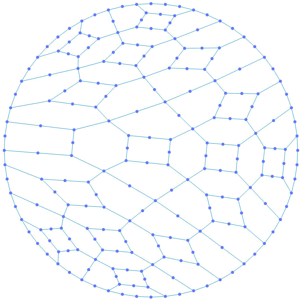
Of course, those tiles don’t look at all like chairs. Why would they? What’s a chair combinatorially? It’s really just a combinatorial octagon. And what does our subdivision rule do? It breaks up a combinatorial octagon into four combinatorial octagons. Nothing about it suggests a chair shape. Or does it? Let’s compute the level 6 subdivision, but color all tiles in the same level-3 supertile with the same color (randomly chosen for each supertile):

tiling = rules.generateTiling("chair", depth = 6)
tutteGraph = tutteEmbeddingE2(tiling)
TutteEmbeddedTilingViewer(
  tiling, 
  tutteGraph, 
  shadedLevel=3 # Shade the level-3 supertiles
).show()

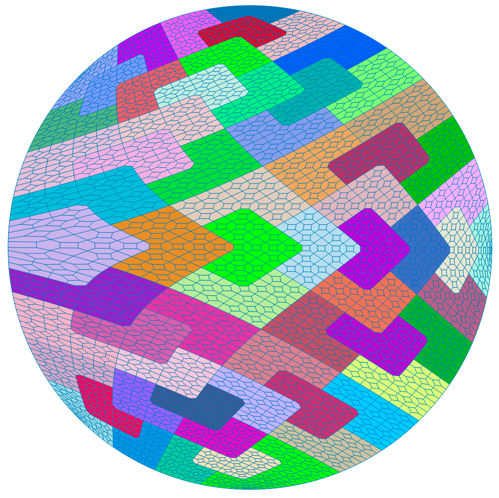
Strange. Those supertiles are looking remarkably chair-like. Remember, we forgot the geometry of the chair tiling completely. Our geometry came from a Tutte embedding which is a generic method of graph drawing that has nothing to do with chair tilings. Then why do the super tiles look like chairs?

…and from combinatorial to conformal…

A Tutte embedding is one way to get geometry from combinatorics. Another way is to find a circle packing. Informally, one variant of the circle packing theorem says that every abstract triangulation of a disk can be realized as a pattern of circles whose contact graph is isormorphic to the 1-skeleton of the original triangulation. (The contact graph of a set of interior disjoint circles is an abstract representation of the incidences between the circles. Each circle is represented as a vertex in the graph and whenever two circles are tangent, their corresponding vertices are connected by an edge.) The figure below shows an example. On the left you see a triangulation with 6 vertices (in this case it’s the 1-skeleton of an octahedron) and on the right (ignoring for the moment the outer circle) you see a pattern of 6 circles whose contact graph is isomorphic to the triangulation on the left.

The circle packing theorems (and I say theorems, because there are really a bunch of related results that deal with triangulations of different homotopy classes as well as different sets of boundary conditions and constraints) are existence and uniqueness theorems. To get to our version of the theorem requires a little bit of hyperbolic geometry.

A digression into hyperbolic geometry.

The hyperbolic plane is a two-dimensional non-Euclidean geometry. A full account of the hyperbolic plane is beyond the scope of this post, but I’ll give a quick crash course. If you are new to this, Henry Segerman and Saul Schleimer have a nice video describing different models for the hyperbolic plane and how they are related by projections in 3-space.

To obtain a non-Euclidean geometry, we throw out Euclid’s fifth postulate which in one incarnation says given a line L and a point p not on L there is a unique line L’ passing through p that is parallel to L. The key phrase here is a unique line. We obtain different geometries by changing the phrase is a unique line to something else. Elliptic geometry, which is spherical geometry except with antipodal points identified, is obtained by replacing is a unique line with is no line. In other words, there are no parallel lines in elliptic geometry! Consider walking in a “straight” line along the earth (and imagine the earth is perfectly spherical). Because of the curvature you will eventually walk all the way around the earth tracing out what we call a great circle and end up back where you started. But from your local point of view, you took the straightest path possible. What you think of as a “line” is really a great circle, but you have to be viewing the sphere at a much more global scale to see this. Key fact: all great circles intersect and thus if you and I start drawing “lines” in starting from different points on the sphere our paths will eventually cross, no matter what.

The hyperbolic plane is obtained by replacing is a unique line in Euclid’s fifth postulate with are infinitely many lines. Just as with the sphere example above we need to have a more global view to really be able to visualize this. What we want is a model of the hyperbolic plane in which we identify the words point and line with some objects that satisfy the normal axioms of geometry–things like two points determines a unique line, two lines either never meet (and are therefore parallel) or intersect at a unique point, etc. as well as our new infinitely-many-parallel-lines version of Euclid’s fifth postulate.

The model we will use is called the Poincaré disk model of the hyperbolic plane. We identify the points in our hyperbolic plane geometry with the points on the interior of the unit disk in the complex plane . A “line” in our geometry is the intersection of the interior of the unit disk with a circle that intersects the boundary at a right angle. Here are two examples.

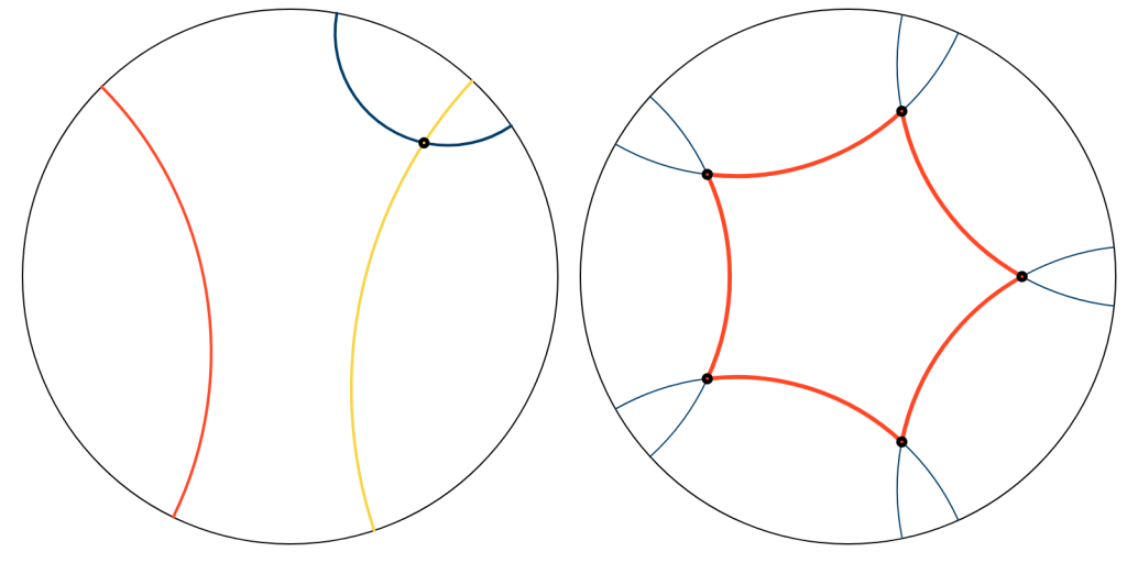
On the left figure above we have two lines, blue and yellow that intersect at a point, but neither intersect the red line. Thus both the yellow line and blue line are parallel to the red. In the right figure above we show a regular pentagon (red) and the supporting lines of its edges (blue).

There is a properly developed notion of distance in the hyperbolic plane. A nice explanation of how to develop this can be found here. For our purposes, only a vague understanding will be required. Recall that in a the Mercator projection of the world distances near the equator appear relatively smaller than distances near the poles–Greenland appears too large. One way to think about this is that starting from the equator as we move up towards the North pole or down towards the South pole our rulers grow so that more of the paper is involved with measuring out a given mile at the top and bottom of the map than in the center. The same thing happens in the Poincare disk model except in reverse. As we move outwards from the origin towards the boundary of the disk our ruler shrinks. In fact, if we measure the distance from the origin to a point that is approaching the boundary of the disk the distance approaches infinity, since we have to put smaller and smaller rulers down as we get closer to the boundary. According to the hyperbolic metric, the boundary of the disk is infinitely far away from any point in the disk.

So distances/lengths are compressing and lines appear to be curves. Is there any sanity to this model? In fact, there is. Two nice features of the Poincare disk are that it preserves angles and circles. In other words, whenever two hyperbolic lines meet at a hyperbolic point, the angle measure between them is exactly the Euclidean angle measure between their corresponding Euclidean circular arcs. Additionally, if we take a hyperbolic point and look at the locus of points a fixed hyperbolic distance of from that point we obtain a hyperbolic circle of radius centered at . If we draw this circle in the hyperbolic plane, its representation to us is a Euclidean circle. However, unless the hyperbolic center is the origin, the Euclidean and hyperbolic centers won’t be the same point. Why is that? Its precisely because the ruler shrinks when it moves near the boundary of the unit disk. Thus the part of the unit disk between the origin and will have a larger ruler than on the other side of . Thus, if we draw a unit circle centered at the origin and translate it outward towards the boundary of the disk, it will appear to us that the center is moving faster towards the disk than the circle (but this is an illusion, just like Greenland being larger than Africa on a Mercator map).

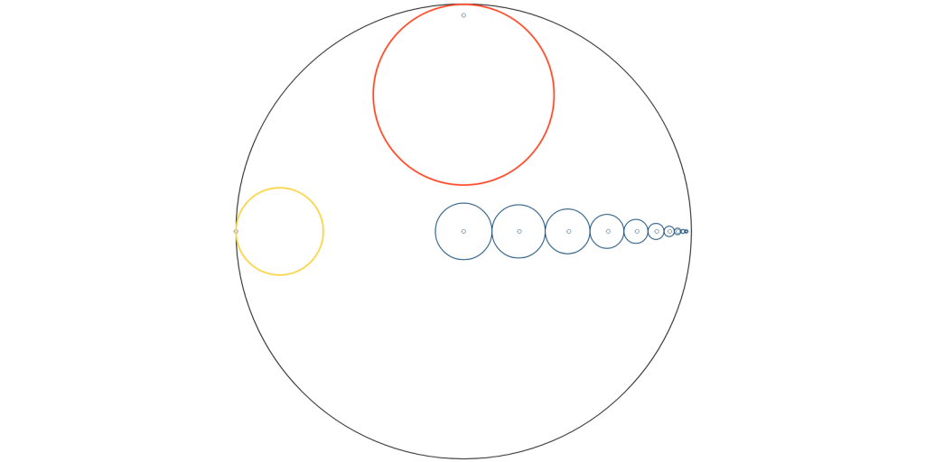
Consider the chain of blue circles in the figure above. Each blue circle has the same hyperbolic radius. From this you can see how as we move towards the boundary the rulers are shrinking. If we wanted them to appear the same size to us, we would need to gradually increase their radii as their centers moved outwards from the origin. The red circle at the top of the disk gives a more extreme example of the compression of our ruler. Note how close the outer boundary the center of this circle (the small dot whose Euclidean coordinates are ) appears to be. All points on the red circle are equidistant from this center point under the hyperbolic metric. Finally, imagine a process in which we move a circle center outwards towards the boundary while increasing its hyperbolic radius so that its Euclidean radius does not change. The limit of such a process is shown in the yellow circle. Here we have a set of points in Euclidean space that are tangent to at a single point. This object is called a horocycle and can be loosely thought of as a circle with a center at infinity and an infinite radius. Horocycles will play a role in our discussion of tilings.

Key Takeaway: Going forward the most important points from this discussion to remember are that Euclidean circles on the interior of the unit disk correspond to hyperbolic circles in the Poincare disk model and Euclidean circles that are tangent to the boundary of the unit disk with interiors contained on the interior of the unit disk correspond to horocycles.

Maximal packings of the hyperbolic plane and conformal maps

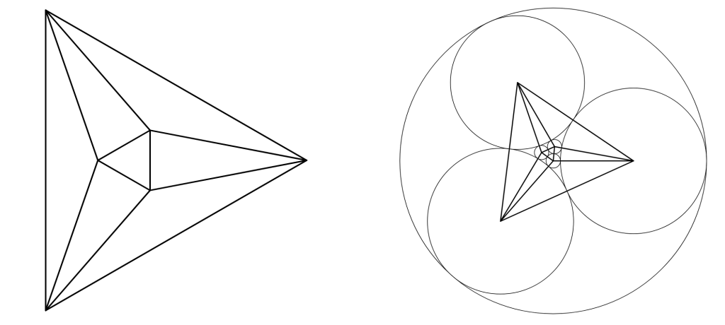
Remember that when we first defined circle packings above, we had an outer circle that I told you to ignore? Let’s draw that same circle packing again, except this time we’re going to connect up hyperbolic circles/horocycle centers with hyperbolic lines/rays/segments instead of Euclidean circle centers with Euclidean segments.

Here our packing is made up of three horocycles (the circles tangent to the unit disk) and three finite circles. Our embedding of the contact graph has the three horocycle centers as points on the boundary of the unit disk. The edge between two neighboring horocycles becomes a hyperbolic line (yellow). The edge between a horocycle and neighboring finite circle becomes a hyberbolic ray (red), and the edge between two neighboring finite circles becomes a hyperbolic line segment (blue). This packing is called a maximal circle packing of the hyperbolic plane because all of the boundary vertices of our abstract triangulation are embedded as horocycles in the packing and all of the interior vertices are embedded as finite circles. We can now state the version of the circle packing theorem that is relevant to our study.

Circle Packing Theorem. Let be a abstract triangulation homeomorphic to a disk. Then there exists a maximal circle packing of the hyperbolic plane whose contact graph is isomorphic to the 1-skeleton of . Furthermore this packing is unique up to Möbius transformations of that map to itself.

Note the uniqueness part of the theorem. The Möbius transformations are the maps that map circles to circles. These maps are also the conformal maps, or angle preserving maps, of to . Suppose is a Möbius transformation that sends the set to itself. Since it maps circles to circles and to , it will also map circular arcs on the interior of the unit disk to circular arcs on the interior of the unit disk. Interpreted in the framework of the Poincaré disk model this means that takes the set of hyperbolic lines to itself. In fact, is a hyperbolic isometry. Denote the hyperbolic distance between two points by . That is a hyperbolic isometry means that for all , . Thus the circle packing theorem states that maximal circle packings of the hyperbolic plane are unique up to hyperbolic isometries!

Infinite conformal tilings

It’s a bit tricky to define infinite conformal tilings in a precise and accessible way. For a reader who is really ready to tackle these fascinating objects, the place to go is [BS17]. My goal here is to give a very brief overview to pique your interest, but the mathematical background required for this section is going to be significantly higher than for the previous sections, and I’m not going to explain the basic concepts. Think of this section as a “why you might want to learn more” to people who already have the appropriate background. If you are without the appropriate background, you may want to skim this section and move on.

Go take a look at at Figure 3 again. The direct limit of our subdivide-and-scale procedure produces a subdivision of the plane into tiles, which we’ll denote by . We’re now going to forget the geometry of this tiling and give the tiling a Riemannian structure via the following construction. For each tile with vertices , we star triangulate the tile by introducing a new vertex and replace the tile with triangles for each $i$ (indices , of course). We place an equilateral metric on each triangle to obtain a Riemannian surface . By the Poincaré-Koebe uniformization theorem this surface is conformally equivalent to either or .

We now apply one further limiting procedure–hex refinement. Hex refinement takes each equilateral triangle and subdivides it by introducing vertices , , and at the midpoints of the edges , , and (respectively) and replaces the triangle with four equilateral triangles , , , and . Suppose we hex refine our structure times. Consider a particular tile in our original tiling . After star triangulation, was subdivided into the triangles . Each hex refinement subdivides each triangle into four, so after applications of hex refinement, our original tile is represented by triangles. Let denote the surface obtained from after refinements. By the uniformization theorem there is a unique conformal map taking to or .

We are now going to look at where this map takes all of the triangles that came from subdividing . These cover some polygonal region of or , which we’ll denote by . Now, let’s take the limit as goes to infinity. The polygons converge to a curvilinear polygon, denoted with vertices whose edges are segments of analytic curves. The original vertices of map directly onto the vertices of . Furthermore the curvilinear polygons satisfy the following 2 conditions.

1. The polygon is conformally regular meaning that there is a conformal map taking to the regular $latexn$-gon in the plane that maps vertices to vertices.
2. For any two neighboring tiles and meeting at an edge , there is an anticonformal reflection between and across the curvilinear edge corresponding to .

The tiling made up of all of the ‘s is called a conformal tiling. In fact, any subdivision of the plane into curvilinear polygons that satisfies conditions 1 and 2 above is called a conformal tiling. It seems a bit remarkable to me that such things exist at all (other than boring examples like square grids) and particularly beautiful that finite subdivision rules can be used to construct them.

Finite quasi-conformal tilings

The conformal tilings described in the last section are mathematically interesting but we would like to be able to see what they look like, which is challenging given that they have infinitely many tiles (some of which, like the chair tiling, have no underlying symmetries to exploit) and on top of that require two different limiting processes to compute.

We’re now going to look at process that gives us just such a drawing. But first let’s get a new tiling, that isn’t our old friend the chair. This is a particularly stunning one called the twisted pentagonal tiling. Unlike the chair tiling, this tiling does not have a corresponding geometric tiling. Thus, I’m going to hand-draw the initial subdivision rule. There’s one prototile, a combinatorial pentagon. We introduce one vertex on its interior and split each of its edges into 3. Finally, we subdivide its interior into five pentagons. Here’s a hand sketch of the rule:

This is purely combinatorial, because there is no way to subdivide a regular pentagon into regular pentagons. Here is the koebepy code for it:

from koebe.algorithms.tiling import *

pent_rules = TilingRules()
pent = pent_rules.createPrototile("pent", tuple("ABCDE"))

pent.addSplitEdgeRules(((("A","B"), ("a", "b")), 
                        (("B","C"), ("c", "d")), 
                        (("C","D"), ("e", "f")),
                        (("D","E"), ("g", "h")), 
                        (("E","A"), ("i", "j"))))

pent.addNewVertexRules(("k"))

pent.addSubtile("pent", tuple("Aabkj"))
pent.addSubtile("pent", tuple("Bcdkb"))
pent.addSubtile("pent", tuple("Cefkd"))
pent.addSubtile("pent", tuple("Dghkf"))
pent.addSubtile("pent", tuple("Eijkh"))

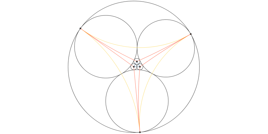
Now, we would like a drawing of this tiling, but instead of using Tutte embeddings, we are going to compute a circle packing. Currently all of our tiles are five-sided, but circle packings require triangulated complexes. To get a triangulated complex we star-triangulate each pentagonal face by introducing a new interior vertex and subdivide the face into triangles by attaching edges from each of the original vertices of the tile to the new vertex. We then compute a circle packing. The left of the figure below shows the result.

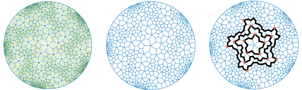
The code for generating the left of figure 14 is below. Changing the showCircles and showTriangulation flags to False produces the center of figure 14. The right was traced by hand in an image editing program. There’s always more to implement. Check out the code, and then let’s talk about the right of figure 14.

pent_tiling = pent_rules.generateTiling("pent", depth = 4)
pent_packing, _ = generateCirclePackingLayout(pent_tiling)
CirclePackedTilingViewer(
    pent_tiling, 
    pent_packing,
    showCircles = True, 
    showTriangulation = True
).show()

In the right of figure 14 I have highlighted the boundaries of supertiles at levels 3, 2, and 1. Think of this as the inverse of the subdivision procedure. I’m aggregating (to use a term from [BS97, BS17]) the subtiles back into their parent super tile to move to a parent level. Notice that we still see a pentagon, but with fractal-like edges stretching between the vertices (red) of each pentagon. There’s a lot of fascinating geometry here, but you’ll have to read [BS97, BS17] for more details. For the twisted pentagonal tiling, in the limit, we get fractal polygons. For some sets of rules, however, this aggregation method does not converge on a fractal. It converges on the shape of the tile in the conformal tiling generated by the rules. The most surprising result, however, comes when we look again at geometric tilings.

…and from conformal back to geometric.

Let’s go back to our old chair tiling again, but this time we’re going to forget its geometry (like we did when we used a Tutte embedding) and use a star-triangulation and a circle packing to obtain a new geometry of the tiling. Take a look at the next figure.

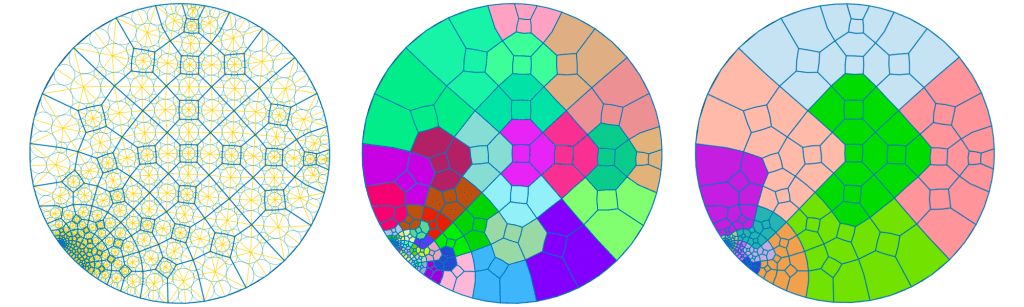
On the left of figure 15 we see the circle packing layout of the level 4 chair tiling. In the middle, I’ve aggregated the level 4 tiles back into their parent tiles from level 3. Already they are beginning to look a bit chair like, except for notches in the at the back of the “seat” of the chair and a notch where the back of the chair meets the floor. The right of the figure shows the aggregate supertiles at level 2. Just 2 levels up from the smallest tiles we are really starting to see chairs emerge and the notches have proportionally gotten smaller. We could imagine computing the level 5 tiling and looking back at the level 2 super tiles (3 levels up this time). We’d again see chairs and again the notches would get smaller.

This raises the question: will the aggregate tiles approach the original geometric tiles? If so this is a rather incredible result. Remember that we threw out the geometry completely and computed a purely combinatorial tiling. We got a new geometry back from circle packing which it would seem is completely arbitrary and unrelated to the original, and yet, it appears that some how the combinatorics of the geometric tiling really encoded the geometry of the tiling as well.

It seems mystical, but this is indeed the case. The following incredible theorem is a corollary of the main result of [KS19]. (Their main result deals with infinite tilings, and the version I’m detailing here deals only with finite tilings.) One fact I’ve glossed over a bit is that circle packings of combinatorial tilings approximate conformal tilings (see [KS19]) and converge to them as the number of subdivisons approaches infinity.

Theorem (Corollary to the Kenyon-Stephenson Theorem [KS19]). Suppose we have a geometric tiling produced by a finite subdivision rule. Let denote a tile produced at level in the conformal tiling that is not incident the boundary. Let denote the set of tiles at level whose aggregate at level is . Then the shape of approaches the shape of original geometric prototile corresponding to as .

In other words, in the limit, those octagons really do turn back into chairs.

Looking forward

I originally intended this post to explain how to use koebepy to produce tilings. I had planned to write a short introduction to tilings as a lead in and if you’ve gotten this far, you’ve seen how short my introduction was. I’m going to leave a technical tutorial on how to actually use the tiling features of koebepy to a future post. There is code below in the Appendix section for several of the figures. For now, please let me know what you think in the comments.

References & Further Reading

[BS97] Bowers, P. and Stephenson, K., 1997. A “regular” pentagonal tiling of the plane. Conformal Geometry and Dynamics of the American Mathematical Society, 1(5), pp.58-86.
[BS17] Bowers, P.L. and Stephenson, K., 2017. Conformal tilings I: foundations, theory, and practice. Conform. Geom. Dyn., 21, pp.1-63.
[CFP01] Cannon, J., Floyd, W. and Parry, W., 2001. Finite subdivision rules. Conformal Geometry and Dynamics of the American Mathematical Society, 5(8), pp.153-196.
[CFP06] Cannon, J., Floyd, W. and Parry, W., 2006. Expansion complexes for finite subdivision rules. I. Conformal Geometry and Dynamics of the American Mathematical Society, 10(4), pp.63-99.
[KS19] Kenyon, R. and Stephenson, K., 2019. Shape convergence for aggregate tiles in conformal tilings. Proceedings of the American Mathematical Society, 147(10), pp.4275-4287.
[S05] Stephenson, K. (2005). Introduction to Circle Packing: The Theory of Discrete Analytic Functions. Cambridge: Cambridge University Press.

Appendix

Code for figure 9 and 12

The first code block produces figure 9. To additionally produce figure 12, append the second code block.

from koebe.geometries.euclidean2 import PointE2, SegmentE2
from koebe.graphics.euclidean2viewer import UnitScaleE2Sketch, PoincareDiskViewer
from koebe.algorithms.incrementalConvexHull import randomConvexHullE3
from koebe.algorithms.tutteEmbeddings import tutteEmbeddingE2

poly = randomConvexHullE3(6) # Generates a random 6 vertex polyhedron
poly.outerFace = poly.faces[0] # Converts one face to the outerface to make it a disk

tutteGraph = tutteEmbeddingE2(poly) # Compute a Tutte embedding

# Show the Tutte embedding
viewer = UnitScaleE2Sketch()
viewer.addAll(
    [SegmentE2(e.aDart.origin.data, e.aDart.twin.origin.data) 
     for e in tutteGraph.edges]
)
viewer.show()

# Compute a maximal packing of the hyperbolic plane
from koebe.algorithms.hypPacker import *

packing, _ = maximalPacking(
    tutteGraph, 
    num_passes=1000
)

# Show the circle packing
viewer = PoincareDiskViewer(600, 600)
viewer.addAll(packing.verts)
viewer.addAll(
    [SegmentE2(PointE2(e.aDart.origin.data.toPoincareCircleE2().center.x, 
                       e.aDart.origin.data.toPoincareCircleE2().center.y), 
               PointE2(e.aDart.dest.data.toPoincareCircleE2().center.x, 
                       e.aDart.dest.data.toPoincareCircleE2().center.y))
    for e in packing.edges]
)
viewer.show()

To produce figure 12 you first run the code above followed by the code below.

from koebe.geometries.hyperbolic2 import PointH2, SegmentH2, LineH2
# Show the circle packing
viewer = PoincareDiskViewer(600, 600)
viewer.addAll(packing.verts)

def sc(z):
    # I haven't implemented SegmentH2/LineH2's between 
    # points at infinity, but the PointH2 class is able to store
    # points at infinity. This function is just scaling points really 
    # close to infinity a bit so they are finite, but appear infinite
    # for drawing purposes. 
    # This is now on my TODO
    if z.coord.modulusSquared > 0.999999999:
        return PointH2(0.9999*z.coord)
    else:
        return z

lineStyle = makeStyle(stroke="#f4d35e", strokeWeight=1.0)
rayStyle = makeStyle(stroke="#f95738", strokeWeight=1.0)
segmentStyle = makeStyle(stroke="#0d3b66", strokeWeight=1.0)
pointStyle = makeStyle(stroke="#000", strokeWeight=2.0)

boundaryVerts = set(packing.outerFace.vertices())
for e in packing.edges:
    u, v = e.endPoints()
    if u in boundaryVerts and v in boundaryVerts:
        viewer.add(SegmentH2(sc(u.data.center), sc(v.data.center)), lineStyle)
    elif u in boundaryVerts or v in boundaryVerts:
        viewer.add(SegmentH2(sc(u.data.center), sc(v.data.center)), rayStyle)
    else:
        viewer.add(SegmentH2(u.data.center, v.data.center), segmentStyle)

viewer.addAll([(v.data.center, pointStyle) for v in packing.verts])

viewer.show()

Code for figure 10 left

from koebe.geometries.hyperbolic2 import *
from koebe.graphics.euclidean2viewer import PoincareDiskViewer, makeStyle

# Create a new Poincare disk viewer
viewer = PoincareDiskViewer(400, 400)

# Create 5 points A, B, C, D, E
A = PointH2.fromComplex(complex(0.5, 0.5))
B = PointH2.fromComplex(complex(0.2, 0.75))
C = PointH2.fromComplex(complex(0.25, -0.15))
D = PointH2.fromComplex(complex(-0.3, -0.4))
E = PointH2.fromComplex(complex(-0.4, 0.25))

# Create some different styles to draw the lines with
blueLine = makeStyle(stroke="#0d3b66", strokeWeight=2.0)
yellowLine = makeStyle(stroke="#f4d35e", strokeWeight=2.0)
redLine = makeStyle(stroke="#f95738", strokeWeight=2.0)
pointStyle = makeStyle(stroke="#000", strokeWeight=3.0)

# Add lines AB, AC, DE and point A to the viewer
viewer.addAll(
  [(LineH2(A, B), blueLine), 
   (LineH2(A, C), yellowLine), 
   (LineH2(D, E), redLine), 
   (A, pointStyle)
  ]
)

# Show the viewer
viewer.show()

Code for figure 10 right

from koebe.geometries.hyperbolic2 import *
from koebe.graphics.euclidean2viewer import PoincareDiskViewer, makeStyle
import math

# Create a poincare disk viewer
viewer = PoincareDiskViewer(400, 400)

# Create 5 points of a regular pentagon centered
# at the origin
A,B,C,D,E = [PointH2.fromComplex(
                    complex(math.cos(2*math.pi*i/5)*0.65,
                            math.sin(2*math.pi*i/5)*0.65))
             for i in range(5)]

# Create some styles for drawing
lineStyle = makeStyle(stroke="#0d3b66", strokeWeight=1.0)
segmentStyle = makeStyle(stroke="#f95738", strokeWeight=3.0)
pointStyle = makeStyle(stroke="#000", strokeWeight=3.0)

# Add the pentagon's supporting lines, segments, and points
# to the viewer. 
viewer.addAll([
    (LineH2(A, B), lineStyle),
    (LineH2(B, C), lineStyle),
    (LineH2(C, D), lineStyle),
    (LineH2(D, E), lineStyle),
    (LineH2(E, A), lineStyle),
    (SegmentH2(A, B), segmentStyle),
    (SegmentH2(B, C), segmentStyle),
    (SegmentH2(C, D), segmentStyle),
    (SegmentH2(D, E), segmentStyle),
    (SegmentH2(E, A), segmentStyle),
    (A, pointStyle), 
    (B, pointStyle), 
    (C, pointStyle), 
    (D, pointStyle), 
    (E, pointStyle)
])

# Show the viewer
viewer.show()

Code for figure 11

from koebe.geometries.hyperbolic2 import *
from koebe.graphics.euclidean2viewer import PoincareDiskViewer, makeStyle
import math

# Converts a length x hyperbolic units along the x-axis to
# the euclidean distance of the point to the origin.
def hypXAxisToEuc(x):
    return CircleH2.withCenterAndHRadius(PointH2(complex(0,0)), x).toPoincareCircleE2().radius

# Create a poincare disk viewer
viewer = PoincareDiskViewer(600, 600)

# Create the circle centers and circles 
As = [PointH2(complex(hypXAxisToEuc(0.5*i), 0)) for i in range(10)]
Cs = [CircleH2.withCenterAndHRadius(A, 0.25) for A in As]

A = PointH2(complex(0, 0.95))
C = CircleH2.withCenterAndHRadius(A, 3.25)

B = PointH2(complex(-0.999999995, 0))
D = CircleH2.withCenterAndHRadius(B, 18.65)

# Create some styles for drawing
circleStyle1 = makeStyle(stroke="#0d3b66", strokeWeight=1.0)
circleStyle2 = makeStyle(stroke="#f95738", strokeWeight=2.0)
circleStyle3 = makeStyle(stroke="#f4d35e", strokeWeight=2.0)
pointStyle = makeStyle(stroke="#0d3b66", strokeWeight=0.5)

# Add the pentagon's supporting lines, segments, and points
# to the viewer. 
viewer.addAll([(A, pointStyle), (C, circleStyle2)])
viewer.addAll([(B, pointStyle), (D, circleStyle3)])
viewer.addAll([(A, pointStyle) for A in As])
viewer.addAll([(C, circleStyle1) for C in Cs])

# Show the viewer
viewer.show()